Categories
Uncategorized

Intuitive Interpretation of Unexpected Binomial Coefficients

This post will give an intuitive interpretation of the presence of the combination formula (which equals the binomial coefficient) in math problem solutions and probability distributions that are seemingly unrelated to combinations. For example, the binomial coefficient shows up in the probability mass function of the binomial distribution and the negative binomial distribution.

Wikipedia has the following definition for combination:

In mathematicscombination is a way of selecting several things out of a larger group, where (unlike permutations) order does not matter. In smaller cases it is possible to count the number of combinations. For example given three fruit, an apple, orange and pear say, there are three combinations of two that can be drawn from this set: an apple and a pear; an apple and an orange; or a pear and an orange. More formally a kcombination of a set S is a subset of k distinct elements of S. If the set has n elements the number of k-combinations is equal to the binomial coefficient

The binomial coefficient indexed by n and k is denoted
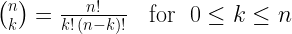
 \tbinom nk. The formula below, for evaluating binomial coefficients, uses factorials.

\binom nk = \frac{n!}{k!\,(n-k)!} \quad \mbox{for }\ 0\leq k\leq n

Categories
Uncategorized

5/19/2011 Quote of the Day

I am going to start posting quotes that I like to my blog. I have been recording quotes that I like for a few years. I will continue to update my list, and use it as a source for quotes to post. A great source for quotes is Bartlett’s Familiar Quotations.

Today’s quote is from Doron Zeilberger.

Whenever I want to learn a new subject, I announce a graduate course in it, since the best way to learn is by teaching. But even better than teaching humans is teaching computers, i.e. program! Since computers will not let you wave your hands and wing it.

Opinion 37 [April 15, 1999]

Also from the same source is the following quote.

In order to understand something really deeply, you should program it.

Opinion 37 [April 15, 1999]

I have never taught a course, so I cannot fully relate to his experience of learning by teaching. However, my unfamiliarity with teaching is one of the reasons that I think that programming is a great way to learn something. While teaching a course requires students, a classroom, a lesson plan, and other constraints, “teaching computers” only requires a computer and a programming language.

Categories
Uncategorized

Installing Your Own Personal WeBWork Server, Part IV

Part IPart IIPart III | Part IV

This series of posts covers the installation of WeBWork. This post, Part IV of the series, will cover how to configure your WeBWork server so that you can access the 20,000 freely available problems.

… Continued from Part III

The last post of this series, Part III, concluded with an image showing the virtual machine and the WeBWork site loaded on my computer. Let’s pick up where we left off, by loading the virtual machine and pointing our browser to http://localhost:14627/webwork2. It is not necessary to log in to the wwadmin account on the Ubuntu machine, as Apache will serve the web pages without logging in. However, it is necessary that the virtual machine is turned on. The window can be minimized to free desktop space. I should mention at this point that I logged into the wwadmin account a few days ago and updated the machine’s software using Ubuntu’s update manager. I am not exactly sure why, but this caused problems with the WeBWork installation (i.e., I received errors when trying to use the site), so I reverted to an earlier snapshot of the virtual machine. I wanted to mention this in case you were considering upgrading the software. An upgrade of the WeBWork software would possibly solve the issues that I was having, but I have not tried this yet.

Categories
Uncategorized

Predicting Y When the Dependent Variable is a Transformation of Y

I am going to try to start posting more frequently. This post covers topics that I’ve been thinking about lately, including model estimation with ordinary least squares (OLS) and forecasting when OLS is used to fit a statistical model with a dependent variable that is a transformation of some variable we wish to forecast.

Suppose we run a regression with the following specification:

Y=\beta_{0}+\beta_{1}X_{1}+\beta_{2}X_{2}+\ldots+\beta_{n}X_{n}+\varepsilon

Let’s assume that the error term is distributed normally, and let’s use OLS to solve for the coefficients in the model. Using a superscript to denote the m observations in the dataset, our m-by-n+1 design matrix \mathbf{X} is

\left[\begin{array}{ccccc} 1 & X_{1}^{(1)} & X_{2}^{(1)} & \cdots & X_{n}^{(1)}\\ 1 & X_{1}^{(2)} & X_{2}^{(2)} & \cdots & X_{n}^{(2)}\\ \vdots & \vdots & \vdots & \ddots & \vdots\\ 1 & X_{1}^{(m)} & X_{2}^{(m)} & \cdots & X_{n}^{(m)}\end{array}\right]

If the coefficient vector is labeled \overrightarrow{\beta} 
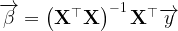
and the vector containing the Y variable’s values is labeled \overrightarrow{y}, then the OLS estimation for the coefficients can be calculated by solving
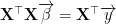
 \mathbf{X}^{\top}\mathbf{X}\overrightarrow{\beta}=\mathbf{X}^{\top}\overrightarrow{y} for \overrightarrow{\beta}.

\overrightarrow{\beta}=\left(\mathbf{X}^{\top}\mathbf{X}\right)^{-1}\mathbf{X}^{\top}\overrightarrow{y}

Now we have a set of coefficients that we can use to predict values of Y when we receive additional observations that have values for our independent variables X1, X2, …, Xn, and no observed values of Y. Everything is fine.

Categories
Uncategorized

Probability Distributions Reference Table

Table Description

I have uploaded a reference table that I created with common probability distributions. Although the same formulas and similar descriptions can be obtained on Wikipedia, I find it useful to have the information contained on one table. The table does not have charts that plot probability density or probability mass functions (PDFs and PMFs) or cumulative distribution functions (CDFs). These charts can be found on Wikipedia or plotted with graphing software using the equations on the table. I find it helpful to look at PDF and CDF plots when learning about the distributions. There might be some closed form CDFs, moment generating functions, or other equations that I omitted from the table. Also, some distributions have various formulations. For example, the four distributions defined below are all very similar, and I imagine that each might be referred to as a negative binomial, although certain specifications are more conventional than others.

  1. A distribution of the number of failures in a sequence of Bernoulli trials, before a specified number of successes.
  2. A distribution of the number of successes in a sequence of Bernoulli trials, before a specified number of failures.
  3. A distribution of the number of successes and failures in a sequence of Bernoulli trials, until a specified number of successes.
  4. A distribution of the number of successes and failures in a sequence of Bernoulli trials, until a specified number of failures.

In cases where there are multiple ways to define a distribution, I either used the definition that I prefer, or gave multiple formulations of the distribution.

I am including a link to both a PDF of the table and an Excel file that has the table and VBA macros for aligning objects. Please let me know if you find any errors.

Links

PDF: Probability-Distributions.pdf
Excel: Probability-Distributions.xlsm