Predicting Y When the Dependent Variable is a Transformation of Y

I am going to try to start posting more frequently. This post covers topics that I’ve been thinking about lately, including model estimation with ordinary least squares (OLS) and forecasting when OLS is used to fit a statistical model with a dependent variable that is a transformation of some variable we wish to forecast.

Suppose we run a regression with the following specification:

$Y=\beta_{0}+\beta_{1}X_{1}+\beta_{2}X_{2}+\ldots+\beta_{n}X_{n}+\varepsilon$

Let’s assume that the error term is distributed normally, and let’s use OLS to solve for the coefficients in the model. Using a superscript to denote the m observations in the dataset, our m-by-n+1 design matrix $\mathbf{X}$ is

$\left[\begin{array}{ccccc} 1 & X_{1}^{(1)} & X_{2}^{(1)} & \cdots & X_{n}^{(1)}\\ 1 & X_{1}^{(2)} & X_{2}^{(2)} & \cdots & X_{n}^{(2)}\\ \vdots & \vdots & \vdots & \ddots & \vdots\\ 1 & X_{1}^{(m)} & X_{2}^{(m)} & \cdots & X_{n}^{(m)}\end{array}\right]$

If the coefficient vector is labeled $\overrightarrow{\beta}$ and the vector containing the Y variable’s values is labeled $\overrightarrow{y}$ , then the OLS estimation for the coefficients can be calculated by solving $\mathbf{X}^{\top}\mathbf{X}\overrightarrow{\beta}=\mathbf{X}^{\top}\overrightarrow{y}$ for $\overrightarrow{\beta}$ .

$\overrightarrow{\beta}=\left(\mathbf{X}^{\top}\mathbf{X}\right)^{-1}\mathbf{X}^{\top}\overrightarrow{y}$

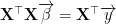
Now we have a set of coefficients that we can use to predict values of Y when we receive additional observations that have values for our independent variables X₁, X₂, …, X_n, and no observed values of Y. Everything is fine.

Now suppose that our original specification was not a good fit for the data and the error terms were not distributed normally. After messing around with the specification, we find that taking the natural logarithm of Y produces a much better fit, and has normally distributed errors. Our new specification is

$\log\left(Y\right)=\beta_{0}+\beta_{1}X_{1}+\beta_{2}X_{2}+\ldots+\beta_{n}X_{n}+\varepsilon$

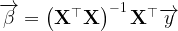
If we repeat the steps described above, we can estimate a new set of coefficients by calculating $\overrightarrow{\beta}=\left(\mathbf{X}^{\top}\mathbf{X}\right)^{-1}\mathbf{X}^{\top}\log\left(\overrightarrow{y}\right)$ where I use $\log\left(\overrightarrow{y}\right)$ to denote the vector that is returned when taking the natural logarithm of each element of $\overrightarrow{y}$ .

We now have a set of coefficients that we can use to predict values of log(Y) when we receive additional observations that have values for our independent variables X₁, X₂, …, X_n, and no observed value of Y. However, we want to predict Y. It may seem natural to just predict Y by taking the exponential function of the predicted value of log(Y). This is where a problem occurs. Our regression is basically returning coefficient values that can be used to express the expected value of the dependent variable, conditioned on the observed values of the independent variables. More formally,

$\mathbb{E}\left[\log\left(Y\right)|X_{1},X_{2},\ldots,X_{n}\right]=\beta_{0}+\beta_{1}X_{1}+\beta_{2}X_{2}+\ldots+\beta_{n}X_{n}$

While it may seem natural to just take the exponential function of the predicted value of log(Y) to predict Y, Jensen’s Inequality implies that $\mathbb{E}\left[f\left(X\right)\right]$ is not necessarily equal to $f\left(\mathbb{E}\left[X\right]\right)$ , where X is a random variable and f is some function of that random variable. We can’t simply take the exponential function of the predicted value of log(Y). Fortunately, for the log-linear model described above, the adjustment is very simple. Since $\log\left(Y\right)|X_{1},X_{2},\ldots,X_{n}$ is distributed normally, we know that $Y|X_{1},X_{2},\ldots,X_{n}$ follows a log-normal distribution (see my prior post—which included a probability distributions reference table—for more details on the log-normal distribution). The expected value of a log-normal distribution is $e^{\mu+\tfrac{1}{2}\sigma^{2}}$ , where $\mu$ is the mean of the underlying normal distribution and $\sigma^{2}$ is its variance. Using this property, we can predict Y by taking the exponential function of the predicted value of log(Y) plus one half of the variance of the error terms in the model, which I will call the mean squared error (MSE).

$\mathbb{E}\left[Y|X_{1},X_{2},\ldots,X_{n}\right]=\exp\left(\mathbb{E}\left[\log\left(Y\right)|X_{1},X_{2},\ldots,X_{n}\right]+\frac{1}{2}MSE\right)$

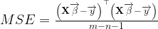
The MSE can be calculated by taking the model’s sum of squared errors, and dividing by the number of observations minus the number of independent variables in the model minus 1.

$MSE=\frac{\left(\mathbf{X}\overrightarrow{\beta}-\overrightarrow{y}\right)^{\top}\left(\mathbf{X}\overrightarrow{\beta}-\overrightarrow{y}\right)}{m-n-1}$

Using $\mathbb{E}\left[\log\left(Y\right)|X_{1},X_{2},\ldots,X_{n}\right]$ and the calculated MSE, we now have our formula for predicting Y.

$\mathbb{E}\left[Y|X_{1},X_{2},\ldots,X_{n}\right]$
$=\exp\left(\beta_{0}+\beta_{1}X_{1}+\beta_{2}X_{2}+\ldots+\beta_{n}X_{n}+\frac{\left(\mathbf{X}\overrightarrow{\beta}-\overrightarrow{y}\right)^{\top}\left(\mathbf{X}\overrightarrow{\beta}-\overrightarrow{y}\right)}{2\cdot\left(m-n-1\right)}\right)$

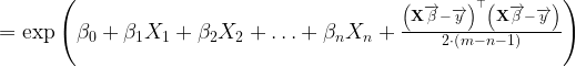
The formula above can be used to predict values of Y using the coefficients estimated by OLS for our log-linear model, and observed values of the independent variables. However, the adjustment is not always so simple. In some cases, more work would be required to calculate how to predict Y when other functions besides the natural logarithm are used to transform Y. In such cases, it might be a good idea to use a different method to model the data, as opposed to trying to transform the variables such that coefficients can be estimated using OLS. While the OLS results often have an intuitive appeal, which can be useful for inference, other models might be more suited for forecasting.

Leave a Reply Cancel reply