statistics – Daniel's Assorted Musings

I am going to try to start posting more frequently. This post covers topics that I’ve been thinking about lately, including model estimation with ordinary least squares (OLS) and forecasting when OLS is used to fit a statistical model with a dependent variable that is a transformation of some variable we wish to forecast.

Suppose we run a regression with the following specification:

$Y=\beta_{0}+\beta_{1}X_{1}+\beta_{2}X_{2}+\ldots+\beta_{n}X_{n}+\varepsilon$

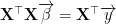
Let’s assume that the error term is distributed normally, and let’s use OLS to solve for the coefficients in the model. Using a superscript to denote the m observations in the dataset, our m-by-n+1 design matrix $\mathbf{X}$ is

$\left[\begin{array}{ccccc} 1 & X_{1}^{(1)} & X_{2}^{(1)} & \cdots & X_{n}^{(1)}\\ 1 & X_{1}^{(2)} & X_{2}^{(2)} & \cdots & X_{n}^{(2)}\\ \vdots & \vdots & \vdots & \ddots & \vdots\\ 1 & X_{1}^{(m)} & X_{2}^{(m)} & \cdots & X_{n}^{(m)}\end{array}\right]$

If the coefficient vector is labeled $\overrightarrow{\beta}$ and the vector containing the Y variable’s values is labeled $\overrightarrow{y}$ , then the OLS estimation for the coefficients can be calculated by solving $\mathbf{X}^{\top}\mathbf{X}\overrightarrow{\beta}=\mathbf{X}^{\top}\overrightarrow{y}$ for $\overrightarrow{\beta}$ .

$\overrightarrow{\beta}=\left(\mathbf{X}^{\top}\mathbf{X}\right)^{-1}\mathbf{X}^{\top}\overrightarrow{y}$

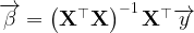
Now we have a set of coefficients that we can use to predict values of Y when we receive additional observations that have values for our independent variables X₁, X₂, …, X_n, and no observed values of Y. Everything is fine.